13.13. Phân loại hình ảnh (CIFAR-10) trên Kaggle

Cho đến nay, chúng tôi đã sử dụng các API cấp cao của các framework deep learning để trực tiếp lấy tập dữ liệu hình ảnh ở định dạng tensor. Tuy nhiên, các tập dữ liệu hình ảnh tùy chỉnh thường có dạng tệp hình ảnh. Trong phần này, chúng ta sẽ bắt đầu từ các tệp hình ảnh thô và sắp xếp, đọc, sau đó chuyển đổi chúng thành định dạng tensor từng bước.

Chúng tôi đã thử nghiệm với tập dữ liệu CIFAR-10 trong Section 13.1, đây là một tập dữ liệu quan trọng trong tầm nhìn máy tính. Trong phần này, chúng tôi sẽ áp dụng kiến thức chúng tôi đã học được trong các phần trước để thực hành cuộc thi Kaggle của phân loại hình ảnh CIFAR-10. Địa chỉ web của cuộc thi là https://www.kaggle.com/c/cifar-10

Fig. 13.13.1 hiển thị thông tin trên trang web của cuộc thi. Để gửi kết quả, bạn cần đăng ký tài khoản Kaggle.

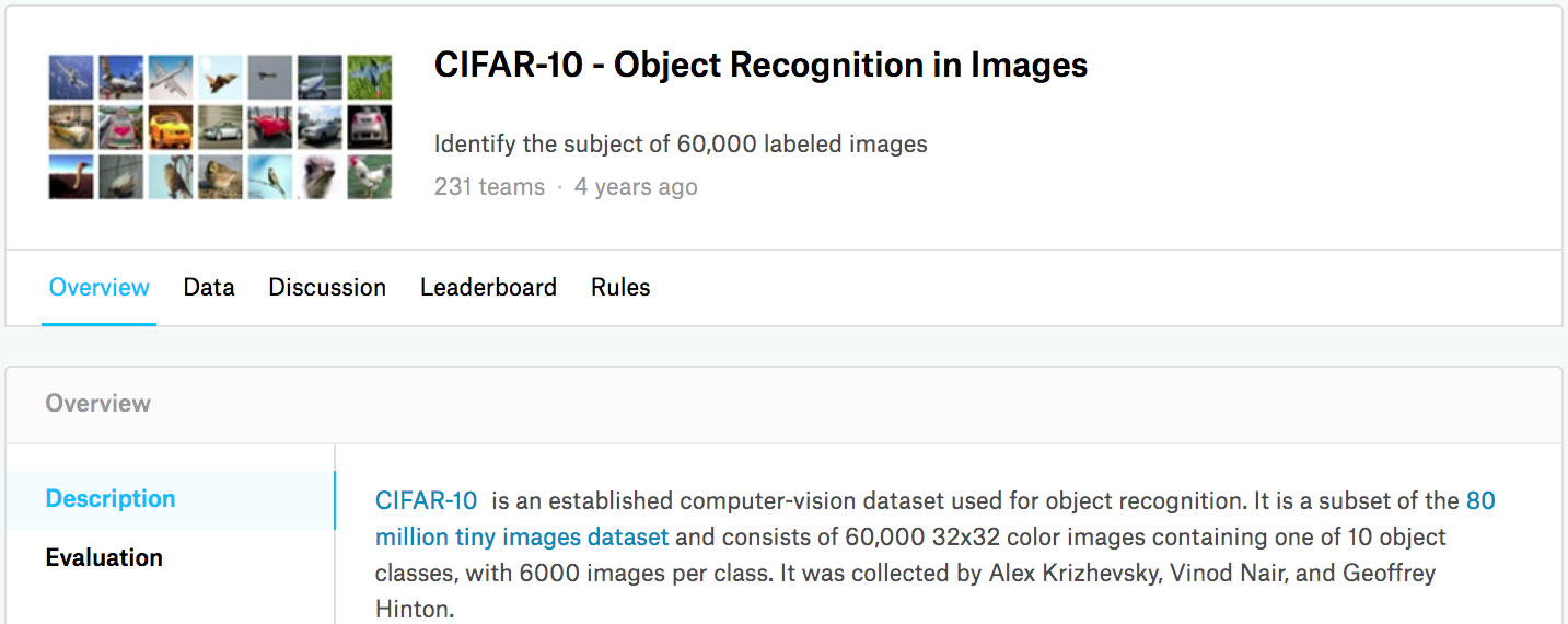
Fig. 13.13.1 CIFAR-10 image classification competition webpage information. The competition dataset can be obtained by clicking the “Data” tab.

mxnetpytorch

import collections
import math
import os
import shutil
import pandas as pd
from mxnet import gluon, init, npx
from mxnet.gluon import nn
from d2l import mxnet as d2l

npx.set_np()

import collections
import math
import os
import shutil
import pandas as pd
import torch
import torchvision
from torch import nn
from d2l import torch as d2l

13.13.1. Lấy và tổ chức tập dữ liệu

Tập dữ liệu cuộc thi được chia thành một bộ đào tạo và một bộ thử nghiệm, có chứa 50000 và 300000 hình ảnh, tương ứng. Trong bộ thử nghiệm, 10000 hình ảnh sẽ được sử dụng để đánh giá, trong khi 290000 hình ảnh còn lại sẽ không được đánh giá: chúng được bao gồm chỉ để làm cho nó khó khăn để lừa dối kết quả được dán nhãn bằng tay của bộ thử nghiệm. Các hình ảnh trong tập dữ liệu này là tất cả các tệp hình ảnh màu png (kênh RGB), có chiều cao và chiều rộng đều là 32 pixel. Các hình ảnh bao gồm tổng cộng 10 loại, cụ thể là máy bay, ô tô, chim, mèo, hươu, chó, ếch, ngựa, thuyền và xe tải. Góc trên bên trái của Fig. 13.13.1 cho thấy một số hình ảnh về máy bay, ô tô và chim trong bộ dữ liệu.

13.13.1.1. Tải xuống tập dữ liệu

Sau khi đăng nhập vào Kaggle, chúng ta có thể nhấp vào tab “Dữ liệu” trên trang web cạnh tranh phân loại hình ảnh CIFAR-10 được hiển thị trong Fig. 13.13.1 và tải xuống tập dữ liệu bằng cách nhấp vào nút “Tải xuống tất cả”. Sau khi giải nén tệp đã tải xuống trong ../data và giải nén train.7z và test.7z bên trong tệp đó, bạn sẽ tìm thấy toàn bộ bộ dữ liệu trong các đường dẫn sau:

• ../data/cifar-10/train/[1-50000].png

• ../data/cifar-10/test/[1-300000].png

• ../data/cifar-10/trainLabels.csv

• ../data/cifar-10/sampleSubmission.csv

trong đó các thư mục train và test chứa các hình ảnh đào tạo và thử nghiệm, tương ứng, trainLabels.csv cung cấp nhãn cho các hình ảnh đào tạo, và sample_submission.csv là một tập tin gửi mẫu.

Để bắt đầu dễ dàng hơn, chúng tôi cung cấp một mẫu quy mô nhỏ của bộ dữ liệu chứa 1000 hình ảnh đào tạo đầu tiên và 5 hình ảnh thử nghiệm ngẫu nhiên. Để sử dụng bộ dữ liệu đầy đủ của cuộc thi Kaggle, bạn cần đặt biến demo sau thành False.

mxnetpytorch

#@save
d2l.DATA_HUB['cifar10_tiny'] = (d2l.DATA_URL + 'kaggle_cifar10_tiny.zip',
                                '2068874e4b9a9f0fb07ebe0ad2b29754449ccacd')

# If you use the full dataset downloaded for the Kaggle competition, set
# `demo` to False
demo = True

if demo:
    data_dir = d2l.download_extract('cifar10_tiny')
else:
    data_dir = '../data/cifar-10/'

Downloading ../data/kaggle_cifar10_tiny.zip from http://d2l-data.s3-accelerate.amazonaws.com/kaggle_cifar10_tiny.zip...

#@save
d2l.DATA_HUB['cifar10_tiny'] = (d2l.DATA_URL + 'kaggle_cifar10_tiny.zip',
                                '2068874e4b9a9f0fb07ebe0ad2b29754449ccacd')

# If you use the full dataset downloaded for the Kaggle competition, set
# `demo` to False
demo = True

if demo:
    data_dir = d2l.download_extract('cifar10_tiny')
else:
    data_dir = '../data/cifar-10/'

Downloading ../data/kaggle_cifar10_tiny.zip from http://d2l-data.s3-accelerate.amazonaws.com/kaggle_cifar10_tiny.zip...

13.13.1.2. Torganizing the Dataset

Chúng ta cần tổ chức các tập dữ liệu để tạo điều kiện cho việc đào tạo và thử nghiệm mô hình. Trước tiên chúng ta hãy đọc các nhãn từ tệp csv. Hàm sau trả về một từ điển mà ánh xạ phần không mở rộng của tên tập tin vào nhãn của nó.

mxnetpytorch

#@save
def read_csv_labels(fname):
    """Read `fname` to return a filename to label dictionary."""
    with open(fname, 'r') as f:
        # Skip the file header line (column name)
        lines = f.readlines()[1:]
    tokens = [l.rstrip().split(',') for l in lines]
    return dict(((name, label) for name, label in tokens))

labels = read_csv_labels(os.path.join(data_dir, 'trainLabels.csv'))
print('# training examples:', len(labels))
print('# classes:', len(set(labels.values())))

# training examples: 1000
# classes: 10

#@save
def read_csv_labels(fname):
    """Read `fname` to return a filename to label dictionary."""
    with open(fname, 'r') as f:
        # Skip the file header line (column name)
        lines = f.readlines()[1:]
    tokens = [l.rstrip().split(',') for l in lines]
    return dict(((name, label) for name, label in tokens))

labels = read_csv_labels(os.path.join(data_dir, 'trainLabels.csv'))
print('# training examples:', len(labels))
print('# classes:', len(set(labels.values())))

# training examples: 1000
# classes: 10

Tiếp theo, chúng ta định nghĩa hàm reorg_train_valid thành chia xác thực được đặt ra khỏi tập đào tạo ban đầu. Đối số valid_ratio trong hàm này là tỷ lệ giữa số ví dụ trong xác thực được đặt thành số ví dụ trong bộ đào tạo ban đầu. Cụ thể hơn, hãy để \(n\) là số lượng hình ảnh của lớp với ít ví dụ nhất, và \(r\) là tỷ lệ. Bộ xác nhận sẽ chia ra \(\max(\lfloor nr\rfloor,1)\) hình ảnh cho mỗi lớp. Hãy để chúng tôi sử dụng valid_ratio=0.1 làm ví dụ. Vì bộ đào tạo ban đầu có 50000 hình ảnh, sẽ có 45000 hình ảnh được sử dụng để đào tạo trong đường train_valid_test/train, trong khi 5000 hình ảnh khác sẽ được chia ra như xác nhận được đặt trong đường train_valid_test/valid. Sau khi tổ chức tập dữ liệu, hình ảnh của cùng một lớp sẽ được đặt dưới cùng một thư mục.

mxnetpytorch

#@save
def copyfile(filename, target_dir):
    """Copy a file into a target directory."""
    os.makedirs(target_dir, exist_ok=True)
    shutil.copy(filename, target_dir)

#@save
def reorg_train_valid(data_dir, labels, valid_ratio):
    """Split the validation set out of the original training set."""
    # The number of examples of the class that has the fewest examples in the
    # training dataset
    n = collections.Counter(labels.values()).most_common()[-1][1]
    # The number of examples per class for the validation set
    n_valid_per_label = max(1, math.floor(n * valid_ratio))
    label_count = {}
    for train_file in os.listdir(os.path.join(data_dir, 'train')):
        label = labels[train_file.split('.')[0]]
        fname = os.path.join(data_dir, 'train', train_file)
        copyfile(fname, os.path.join(data_dir, 'train_valid_test',
                                     'train_valid', label))
        if label not in label_count or label_count[label] < n_valid_per_label:
            copyfile(fname, os.path.join(data_dir, 'train_valid_test',
                                         'valid', label))
            label_count[label] = label_count.get(label, 0) + 1
        else:
            copyfile(fname, os.path.join(data_dir, 'train_valid_test',
                                         'train', label))
    return n_valid_per_label

#@save
def copyfile(filename, target_dir):
    """Copy a file into a target directory."""
    os.makedirs(target_dir, exist_ok=True)
    shutil.copy(filename, target_dir)

#@save
def reorg_train_valid(data_dir, labels, valid_ratio):
    """Split the validation set out of the original training set."""
    # The number of examples of the class that has the fewest examples in the
    # training dataset
    n = collections.Counter(labels.values()).most_common()[-1][1]
    # The number of examples per class for the validation set
    n_valid_per_label = max(1, math.floor(n * valid_ratio))
    label_count = {}
    for train_file in os.listdir(os.path.join(data_dir, 'train')):
        label = labels[train_file.split('.')[0]]
        fname = os.path.join(data_dir, 'train', train_file)
        copyfile(fname, os.path.join(data_dir, 'train_valid_test',
                                     'train_valid', label))
        if label not in label_count or label_count[label] < n_valid_per_label:
            copyfile(fname, os.path.join(data_dir, 'train_valid_test',
                                         'valid', label))
            label_count[label] = label_count.get(label, 0) + 1
        else:
            copyfile(fname, os.path.join(data_dir, 'train_valid_test',
                                         'train', label))
    return n_valid_per_label

Hàm reorg_test bên dưới tổ chức bộ thử nghiệm để tải dữ liệu trong quá trình dự đoán.

mxnetpytorch

#@save
def reorg_test(data_dir):
    """Organize the testing set for data loading during prediction."""
    for test_file in os.listdir(os.path.join(data_dir, 'test')):
        copyfile(os.path.join(data_dir, 'test', test_file),
                 os.path.join(data_dir, 'train_valid_test', 'test',
                              'unknown'))

#@save
def reorg_test(data_dir):
    """Organize the testing set for data loading during prediction."""
    for test_file in os.listdir(os.path.join(data_dir, 'test')):
        copyfile(os.path.join(data_dir, 'test', test_file),
                 os.path.join(data_dir, 'train_valid_test', 'test',
                              'unknown'))

Cuối cùng, chúng ta sử dụng một hàm để invoke read_csv_labels, reorg_train_valid, và reorg_test functions được định nghĩa ở trên.

mxnetpytorch

def reorg_cifar10_data(data_dir, valid_ratio):
    labels = read_csv_labels(os.path.join(data_dir, 'trainLabels.csv'))
    reorg_train_valid(data_dir, labels, valid_ratio)
    reorg_test(data_dir)

def reorg_cifar10_data(data_dir, valid_ratio):
    labels = read_csv_labels(os.path.join(data_dir, 'trainLabels.csv'))
    reorg_train_valid(data_dir, labels, valid_ratio)
    reorg_test(data_dir)

Ở đây chúng tôi chỉ đặt kích thước lô thành 32 cho mẫu quy mô nhỏ của tập dữ liệu. Khi đào tạo và thử nghiệm tập dữ liệu hoàn chỉnh của cuộc thi Kaggle, batch_size nên được đặt thành một số nguyên lớn hơn, chẳng hạn như 128. Chúng tôi chia ra 10% các ví dụ đào tạo là xác nhận được thiết lập để điều chỉnh các siêu tham số.

mxnetpytorch

batch_size = 32 if demo else 128
valid_ratio = 0.1
reorg_cifar10_data(data_dir, valid_ratio)

batch_size = 32 if demo else 128
valid_ratio = 0.1
reorg_cifar10_data(data_dir, valid_ratio)

13.13.2. Image Augmentation

Chúng tôi sử dụng nâng hình ảnh để giải quyết overfitting. Ví dụ, hình ảnh có thể được lật theo chiều ngang ngẫu nhiên trong quá trình đào tạo. Chúng tôi cũng có thể thực hiện tiêu chuẩn hóa cho ba kênh RGB của hình ảnh màu. Dưới đây liệt kê một số hoạt động mà bạn có thể tinh chỉnh.

mxnetpytorch

transform_train = gluon.data.vision.transforms.Compose([
    # Scale the image up to a square of 40 pixels in both height and width
    gluon.data.vision.transforms.Resize(40),
    # Randomly crop a square image of 40 pixels in both height and width to
    # produce a small square of 0.64 to 1 times the area of the original
    # image, and then scale it to a square of 32 pixels in both height and
    # width
    gluon.data.vision.transforms.RandomResizedCrop(32, scale=(0.64, 1.0),
                                                   ratio=(1.0, 1.0)),
    gluon.data.vision.transforms.RandomFlipLeftRight(),
    gluon.data.vision.transforms.ToTensor(),
    # Standardize each channel of the image
    gluon.data.vision.transforms.Normalize([0.4914, 0.4822, 0.4465],
                                           [0.2023, 0.1994, 0.2010])])

transform_train = torchvision.transforms.Compose([
    # Scale the image up to a square of 40 pixels in both height and width
    torchvision.transforms.Resize(40),
    # Randomly crop a square image of 40 pixels in both height and width to
    # produce a small square of 0.64 to 1 times the area of the original
    # image, and then scale it to a square of 32 pixels in both height and
    # width
    torchvision.transforms.RandomResizedCrop(32, scale=(0.64, 1.0),
                                                   ratio=(1.0, 1.0)),
    torchvision.transforms.RandomHorizontalFlip(),
    torchvision.transforms.ToTensor(),
    # Standardize each channel of the image
    torchvision.transforms.Normalize([0.4914, 0.4822, 0.4465],
                                     [0.2023, 0.1994, 0.2010])])

Trong quá trình thử nghiệm, chúng tôi chỉ thực hiện tiêu chuẩn hóa trên hình ảnh để loại bỏ sự ngẫu nhiên trong kết quả đánh giá.

mxnetpytorch

transform_test = gluon.data.vision.transforms.Compose([
    gluon.data.vision.transforms.ToTensor(),
    gluon.data.vision.transforms.Normalize([0.4914, 0.4822, 0.4465],
                                           [0.2023, 0.1994, 0.2010])])

transform_test = torchvision.transforms.Compose([
    torchvision.transforms.ToTensor(),
    torchvision.transforms.Normalize([0.4914, 0.4822, 0.4465],
                                     [0.2023, 0.1994, 0.2010])])

13.13.3. Đọc tập dữ liệu

Tiếp theo, chúng ta đọc tập dữ liệu có tổ chức bao gồm các tập tin hình ảnh thô. Mỗi ví dụ bao gồm một hình ảnh và một nhãn.

mxnetpytorch

train_ds, valid_ds, train_valid_ds, test_ds = [
    gluon.data.vision.ImageFolderDataset(
        os.path.join(data_dir, 'train_valid_test', folder))
    for folder in ['train', 'valid', 'train_valid', 'test']]

train_ds, train_valid_ds = [torchvision.datasets.ImageFolder(
    os.path.join(data_dir, 'train_valid_test', folder),
    transform=transform_train) for folder in ['train', 'train_valid']]

valid_ds, test_ds = [torchvision.datasets.ImageFolder(
    os.path.join(data_dir, 'train_valid_test', folder),
    transform=transform_test) for folder in ['valid', 'test']]

Trong quá trình đào tạo, chúng ta cần chỉ định tất cả các thao tác nâng hình ảnh được xác định ở trên. Khi bộ xác thực được sử dụng để đánh giá mô hình trong quá trình điều chỉnh siêu tham số, không nên giới thiệu tính ngẫu nhiên từ việc tăng hình ảnh. Trước khi dự đoán cuối cùng, chúng tôi đào tạo mô hình trên bộ đào tạo kết hợp và bộ xác nhận để tận dụng tối đa tất cả dữ liệu được dán nhãn.

mxnetpytorch

train_iter, train_valid_iter = [gluon.data.DataLoader(
    dataset.transform_first(transform_train), batch_size, shuffle=True,
    last_batch='discard') for dataset in (train_ds, train_valid_ds)]

valid_iter = gluon.data.DataLoader(
    valid_ds.transform_first(transform_test), batch_size, shuffle=False,
    last_batch='discard')

test_iter = gluon.data.DataLoader(
    test_ds.transform_first(transform_test), batch_size, shuffle=False,
    last_batch='keep')

train_iter, train_valid_iter = [torch.utils.data.DataLoader(
    dataset, batch_size, shuffle=True, drop_last=True)
    for dataset in (train_ds, train_valid_ds)]

valid_iter = torch.utils.data.DataLoader(valid_ds, batch_size, shuffle=False,
                                         drop_last=True)

test_iter = torch.utils.data.DataLoader(test_ds, batch_size, shuffle=False,
                                        drop_last=False)

13.13.4. Xác định Mẫu

mxnetpytorch

Ở đây, chúng tôi xây dựng các khối còn lại dựa trên lớp HybridBlock, hơi khác so với việc triển khai được mô tả trong Section 7.6. Điều này là để cải thiện hiệu quả tính toán.

class Residual(nn.HybridBlock):
    def __init__(self, num_channels, use_1x1conv=False, strides=1, **kwargs):
        super(Residual, self).__init__(**kwargs)
        self.conv1 = nn.Conv2D(num_channels, kernel_size=3, padding=1,
                               strides=strides)
        self.conv2 = nn.Conv2D(num_channels, kernel_size=3, padding=1)
        if use_1x1conv:
            self.conv3 = nn.Conv2D(num_channels, kernel_size=1,
                                   strides=strides)
        else:
            self.conv3 = None
        self.bn1 = nn.BatchNorm()
        self.bn2 = nn.BatchNorm()

    def hybrid_forward(self, F, X):
        Y = F.npx.relu(self.bn1(self.conv1(X)))
        Y = self.bn2(self.conv2(Y))
        if self.conv3:
            X = self.conv3(X)
        return F.npx.relu(Y + X)

Tiếp theo, chúng tôi xác định mô hình ResNet-18.

def resnet18(num_classes):
    net = nn.HybridSequential()
    net.add(nn.Conv2D(64, kernel_size=3, strides=1, padding=1),
            nn.BatchNorm(), nn.Activation('relu'))

    def resnet_block(num_channels, num_residuals, first_block=False):
        blk = nn.HybridSequential()
        for i in range(num_residuals):
            if i == 0 and not first_block:
                blk.add(Residual(num_channels, use_1x1conv=True, strides=2))
            else:
                blk.add(Residual(num_channels))
        return blk

    net.add(resnet_block(64, 2, first_block=True),
            resnet_block(128, 2),
            resnet_block(256, 2),
            resnet_block(512, 2))
    net.add(nn.GlobalAvgPool2D(), nn.Dense(num_classes))
    return net

Chúng tôi sử dụng khởi tạo Xavier được mô tả trong Section 4.8.2.2 trước khi đào tạo bắt đầu.

def get_net(devices):
    num_classes = 10
    net = resnet18(num_classes)
    net.initialize(ctx=devices, init=init.Xavier())
    return net

loss = gluon.loss.SoftmaxCrossEntropyLoss()

Chúng tôi xác định mô hình ResNet-18 được mô tả trong Section 7.6.

def get_net():
    num_classes = 10
    net = d2l.resnet18(num_classes, 3)
    return net

loss = nn.CrossEntropyLoss(reduction="none")

13.13.5. Xác định đào tạo chức năng

Chúng tôi sẽ chọn các mô hình và điều chỉnh các siêu tham số theo hiệu suất của mô hình trên bộ xác thực. Sau đây, chúng tôi xác định hàm đào tạo mô hình train.

mxnetpytorch

def train(net, train_iter, valid_iter, num_epochs, lr, wd, devices, lr_period,
          lr_decay):
    trainer = gluon.Trainer(net.collect_params(), 'sgd',
                            {'learning_rate': lr, 'momentum': 0.9, 'wd': wd})
    num_batches, timer = len(train_iter), d2l.Timer()
    legend = ['train loss', 'train acc']
    if valid_iter is not None:
        legend.append('valid acc')
    animator = d2l.Animator(xlabel='epoch', xlim=[1, num_epochs],
                            legend=legend)
    for epoch in range(num_epochs):
        metric = d2l.Accumulator(3)
        if epoch > 0 and epoch % lr_period == 0:
            trainer.set_learning_rate(trainer.learning_rate * lr_decay)
        for i, (features, labels) in enumerate(train_iter):
            timer.start()
            l, acc = d2l.train_batch_ch13(
                net, features, labels.astype('float32'), loss, trainer,
                devices, d2l.split_batch)
            metric.add(l, acc, labels.shape[0])
            timer.stop()
            if (i + 1) % (num_batches // 5) == 0 or i == num_batches - 1:
                animator.add(epoch + (i + 1) / num_batches,
                             (metric[0] / metric[2], metric[1] / metric[2],
                              None))
        if valid_iter is not None:
            valid_acc = d2l.evaluate_accuracy_gpus(net, valid_iter,
                                                   d2l.split_batch)
            animator.add(epoch + 1, (None, None, valid_acc))
    measures = (f'train loss {metric[0] / metric[2]:.3f}, '
                f'train acc {metric[1] / metric[2]:.3f}')
    if valid_iter is not None:
        measures += f', valid acc {valid_acc:.3f}'
    print(measures + f'\n{metric[2] * num_epochs / timer.sum():.1f}'
          f' examples/sec on {str(devices)}')

def train(net, train_iter, valid_iter, num_epochs, lr, wd, devices, lr_period,
          lr_decay):
    trainer = torch.optim.SGD(net.parameters(), lr=lr, momentum=0.9,
                              weight_decay=wd)
    scheduler = torch.optim.lr_scheduler.StepLR(trainer, lr_period, lr_decay)
    num_batches, timer = len(train_iter), d2l.Timer()
    legend = ['train loss', 'train acc']
    if valid_iter is not None:
        legend.append('valid acc')
    animator = d2l.Animator(xlabel='epoch', xlim=[1, num_epochs],
                            legend=legend)
    net = nn.DataParallel(net, device_ids=devices).to(devices[0])
    for epoch in range(num_epochs):
        net.train()
        metric = d2l.Accumulator(3)
        for i, (features, labels) in enumerate(train_iter):
            timer.start()
            l, acc = d2l.train_batch_ch13(net, features, labels,
                                          loss, trainer, devices)
            metric.add(l, acc, labels.shape[0])
            timer.stop()
            if (i + 1) % (num_batches // 5) == 0 or i == num_batches - 1:
                animator.add(epoch + (i + 1) / num_batches,
                             (metric[0] / metric[2], metric[1] / metric[2],
                              None))
        if valid_iter is not None:
            valid_acc = d2l.evaluate_accuracy_gpu(net, valid_iter)
            animator.add(epoch + 1, (None, None, valid_acc))
        scheduler.step()
    measures = (f'train loss {metric[0] / metric[2]:.3f}, '
                f'train acc {metric[1] / metric[2]:.3f}')
    if valid_iter is not None:
        measures += f', valid acc {valid_acc:.3f}'
    print(measures + f'\n{metric[2] * num_epochs / timer.sum():.1f}'
          f' examples/sec on {str(devices)}')

13.13.6. Đào tạo và xác thực mô hình

Bây giờ, chúng ta có thể đào tạo và xác thực mô hình. Tất cả các siêu tham số sau đây có thể được điều chỉnh. Ví dụ, chúng ta có thể tăng số lượng kỷ nguyên. Khi lr_period và lr_decay được đặt thành 4 và 0,9, tương ứng, tốc độ học tập của thuật toán tối ưu hóa sẽ được nhân với 0,9 sau mỗi 4 kỷ nguyên. Chỉ để dễ dàng trình diễn, chúng tôi chỉ đào tạo 20 kỷ nguyên ở đây.

mxnetpytorch

devices, num_epochs, lr, wd = d2l.try_all_gpus(), 20, 0.02, 5e-4
lr_period, lr_decay, net = 4, 0.9, get_net(devices)
net.hybridize()
train(net, train_iter, valid_iter, num_epochs, lr, wd, devices, lr_period,
      lr_decay)

train loss 0.726, train acc 0.757, valid acc 0.438
370.7 examples/sec on [gpu(0), gpu(1)]

devices, num_epochs, lr, wd = d2l.try_all_gpus(), 20, 2e-4, 5e-4
lr_period, lr_decay, net = 4, 0.9, get_net()
train(net, train_iter, valid_iter, num_epochs, lr, wd, devices, lr_period,
      lr_decay)

train loss 0.736, train acc 0.749, valid acc 0.422
898.8 examples/sec on [device(type='cuda', index=0), device(type='cuda', index=1)]

13.13.7. Phân loại bộ thử nghiệm và gửi kết quả trên Kaggle

Sau khi có được một mô hình đầy hứa hẹn với các siêu tham số, chúng tôi sử dụng tất cả dữ liệu được dán nhãn (bao gồm cả bộ xác thực) để đào tạo lại mô hình và phân loại bộ thử nghiệm.

mxnetpytorch

net, preds = get_net(devices), []
net.hybridize()
train(net, train_valid_iter, None, num_epochs, lr, wd, devices, lr_period,
      lr_decay)

for X, _ in test_iter:
    y_hat = net(X.as_in_ctx(devices[0]))
    preds.extend(y_hat.argmax(axis=1).astype(int).asnumpy())
sorted_ids = list(range(1, len(test_ds) + 1))
sorted_ids.sort(key=lambda x: str(x))
df = pd.DataFrame({'id': sorted_ids, 'label': preds})
df['label'] = df['label'].apply(lambda x: train_valid_ds.synsets[x])
df.to_csv('submission.csv', index=False)

train loss 0.950, train acc 0.657
830.9 examples/sec on [gpu(0), gpu(1)]

net, preds = get_net(), []
train(net, train_valid_iter, None, num_epochs, lr, wd, devices, lr_period,
      lr_decay)

for X, _ in test_iter:
    y_hat = net(X.to(devices[0]))
    preds.extend(y_hat.argmax(dim=1).type(torch.int32).cpu().numpy())
sorted_ids = list(range(1, len(test_ds) + 1))
sorted_ids.sort(key=lambda x: str(x))
df = pd.DataFrame({'id': sorted_ids, 'label': preds})
df['label'] = df['label'].apply(lambda x: train_valid_ds.classes[x])
df.to_csv('submission.csv', index=False)

train loss 0.755, train acc 0.721
1165.8 examples/sec on [device(type='cuda', index=0), device(type='cuda', index=1)]

Mã trên sẽ tạo ra một tập tin submission.csv, có định dạng đáp ứng yêu cầu của cuộc thi Kaggle. Phương pháp gửi kết quả cho Kaggle tương tự như trong Section 4.10.

13.13.8. Tóm tắt

• Chúng ta có thể đọc các bộ dữ liệu chứa các tệp hình ảnh thô sau khi sắp xếp chúng thành định dạng cần thiết.

mxnetpytorch

• Chúng ta có thể sử dụng các mạng thần kinh phức tạp, nâng hình ảnh và lập trình lai trong một cuộc thi phân loại hình ảnh.

• Chúng ta có thể sử dụng mạng thần kinh phức tạp và nâng hình ảnh trong một cuộc thi phân loại hình ảnh.

13.13.9. Bài tập

1. Sử dụng bộ dữ liệu CIFAR-10 hoàn chỉnh cho cuộc thi Kaggle này. Đặt các siêu tham số là batch_size = 128, num_epochs = 100, lr = 0.1, lr_period = 50 và lr_decay = 0.1. Xem độ chính xác và thứ hạng bạn có thể đạt được trong cuộc thi này. Bạn có thể cải thiện thêm chúng?

2. Độ chính xác nào bạn có thể nhận được khi không sử dụng nâng hình ảnh?

mxnetpytorch

Discussions

Discussions